
Key Steps in Flow Modeling for Pressure Drop Calculation:
- Pressure drop calculation in gas pipes using software like Air Flow toolstypically involves modeling the flow of gas through a pipe network and computing the pressure losses due to friction, fittings, and other resistances.
- Here’s a step-by-step guide to understanding how it works:

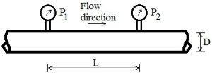
Pressure drop calculation schematic
Key Inputs Required
- Pipe Characteristics:
- Length of each pipe segment (m or ft).
- Inner diameter of the pipe (mm or inches).
- Material and roughness (e.g., steel, PVC, etc.).
- Number and type of fittings (elbows, valves, tees, etc.).
- Gas Properties:
- Type of gas (e.g., air, natural gas, CO₂, etc.).
- Density (ρ) in kg/m³ or lb/ft³.
- Viscosity (μ) in Pa·s or lb/(ft·s).
- Flow Parameters:
- Flow rate (Q) in m³/s or CFM.
- Pressure and temperature of the gas at the inlet (to account for Compressibility).
- Boundary Conditions:
- Inlet pressure (e.g., supply pressure in kPa or psi).
- Desired outlet pressure or flow rate at the endpoint.
Steps Performed by the Software
- Determine the Reynolds Number (ReRe):
- Used to identify flow regime (laminar or turbulent).
Re=ρvD/μwhere:
- v: Flow velocity (m/s).
- D: Pipe diameter (m).
- Calculate the Friction Factor (f):
- For laminar flow (Re<2000): f=64/Ref
- For turbulent flow (Re>4000):
- Use the Cole brook -White equation
- Calculate Pressure Drop Due to Friction:
- Using the Darcy-Weisbach equation: ΔPf=f⋅LD⋅ρv^2/2gD
Darcy Weeisbach Equation for Pressure Drop Determination
- Using the Darcy-Weisbach equation: ΔPf=f⋅LD⋅ρv^2/2gD
- Include Pressure Loss from Fittings and Components:
- Use K-values for each fitting and calculate: ΔP=K⋅ρv^2\Delta P
- Account for Compressibility:
- For gases, adjust calculations for varying density: ΔP=Z/R*P/⋅T⋅ΔP_ideal
- where Z is the Compressibility factor, RR is the gas constant, and T is temperature.
- Iterate Through Network:
- The software calculates pressure losses at each segment, adjusting for flow splits, junctions, and network complexity.

Outputs from the Software
- Pressure Drop:
- Total pressure loss from inlet to outlet.
- Intermediate pressures at key points.
- Flow Distribution:
- Flow rates in each branch of the network.
- Velocity and Reynolds Number:
- For each pipe segment.
- Energy Loss:
- Quantification of energy dissipation.
- Refer the webpage for pressure drop calculations in pipes and fitting
Assumption for Pressure drop calculation in Gas Pipes
- FT Fathom (Applied Flow Technology Fathom) is a powerful software tool for modeling pressure drop and flow distribution in incompressible or low-compressibility fluid systems, including gas networks under specific conditions.
- The assumptions used in AFT Fathom calculations are crucial for understanding the results’ limitations and accuracy.
- Here are the key assumptions typically made during pressure drop calculations:

Fluid Assumptions
- Incompressible Flow:
- AFT Fathom assumes incompressible flow for most calculations. For gases, this means density is considered constant unless the optional Compressible Flow module is activated.
- Uniform Properties:
- Fluid properties (density, viscosity) are assumed to remain constant throughout the system unless the fluid temperature or composition changes are explicitly modeled.
- Single-Phase Flow:
- AFT Fathom assumes a single-phase fluid system with no phase change (e.g., no condensation or cavitation).
Flow Assumptions
- Steady-State Flow:
- The flow is assumed to be steady, meaning there are no temporal changes in velocity, pressure, or flow rate within the system.
- Fully Developed Flow:
- The flow is treated as fully developed in straight pipes, and entrance effects are generally neglected unless specifically modeled.
- No Flow Separation:
- Flow separation in fittings (e.g., at sharp bends or sudden expansions) is represented by empirical loss coefficients and is not explicitly modeled.
Pipe and Component Assumptions
- Uniform Geometry:
- Pipe segments are assumed to have a constant diameter, length, and roughness unless specified otherwise.
- Surface Roughness:
- The pipe roughness is considered uniform and is based on the material data provided by the user or the software database.
- Empirical Loss Coefficients:
- Losses due to fittings, valves, and other components are calculated using standard empirical KK-values unless custom values are specified.
- Negligible Elevation Effects:
- Changes in elevation are accounted for if specified, but for gas systems under low-pressure conditions, they are often negligible compared to friction and fitting losses.
Thermal and Compressibility Assumptions
- Isothermal Flow:
- Gas flow is generally modeled as isothermal unless a heat transfer module or energy balance is included.
- Low Compressibility:
- For gases, the system must meet the low-compressibility assumption (pressure changes less than 10–15% of the absolute pressure) unless the optional Compressible Flow Module is used.
Boundary Conditions
- Fixed Boundary Conditions:
- The inlet pressure, outlet pressure, or flow rates at certain points are fixed and must be specified correctly for the solution to converge.
- Conservation of Mass:
- AFT Fathom assumes mass conservation throughout the system, with all inflows and outflows balanced.
- Conservation of Energy:
- Pressure losses due to friction, fittings, and elevation changes are calculated based on the total energy balance.
Computational Assumptions
- Empirical Models:
- Friction factors are calculated using the Darcy-Weisbach equation, with the friction factor determined by the Colebrook-White equation or similar empirical relationships.
- Linear or Nonlinear Solution Techniques:
- AFT Fathom uses iterative numerical methods to solve the system equations. It assumes convergence when the solution meets a specified tolerance.
- No Leakage:
- The system is assumed to be leak-free unless leaks are explicitly modeled.
Optional Features and Assumptions with Modules
- Compressible Flow Module:
- For high-pressure gas systems, the compressibility effects are included by solving the full energy equation and using variable gas properties.
- Heat Transfer Module:
- If heat transfer is activated, the fluid temperature is allowed to vary, and thermal effects are considered.
- Pump and Valve Models:
- Pumps and valves are modeled using manufacturer data or standard performance curves, which are assumed accurate.
Key Considerations for Accurate Results
- Ensure that the input data (pipe lengths, diameters, roughness, flow rates, pressures, and fitting details) are precise.
- For gas systems, verify whether the low-compressibility assumption is valid or if the Compressible Flow Module is required.
- Use proper boundary conditions to represent the physical system accurately.
Simulation Tools for Pressure Drop Calculations

Advantages of Using Air Flow Technology Software
- Accuracy: Incorporates all significant factors, including fittings, flow regime, and compressibility.
- Visualization: Offers graphical representation of pressure and velocity profiles.
- Efficiency: Automates iterative calculations for complex networks.
- Customization: Allows specification of custom fittings, pipes, and gas properties.
Application Areas
- Natural gas distribution systems.
- Compressed air piping networks.
- HVAC ducting for gases.
- Industrial gas transport.
Pressure drop calculation using ASHRAE
- Calculating pressure drop in HVAC systems using ASHRAE guidelines typically involves evaluating frictional losses in ductwork and fittings, as well as accounting for velocity and pressure changes.
- Here’s a step-by-step guide to performing this calculation based on ASHRAE standards:
Step 1: Gather Required Inputs
- Airflow rate (): In cubic feet per minute (CFM) or cubic meters per second (m³/s).
- Duct size and shape: Dimensions of the duct (rectangular or round).
- Duct material: Material type to determine the roughness factor.
- Duct length (): Total length of the duct in feet or meters.
- Air density (ρ): At design temperature and pressure.
- Air velocity (V): Typically calculated as V=Q/A , where A is the cross-sectional area of the duct.
- Equivalent length of fittings (): ASHRAE provides tables for equivalent lengths for elbows, tees, dampers, etc.
Step 2: Use the Darcy-Weisbach Equation
The total pressure drop (ΔP) is calculated using the Darcy-Weisbach Equation
Step 3: Calculate Friction Factor ()
- Calculate the Reynolds number (Re):
- Determine ff based on ReRe and relative roughness (ϵ/D)
-
Dynamic losses from fittings and transitions are added to the frictional losses.
- Combine All Losses
Tools for Calculation
- ASHRAE Handbook of Fundamentals: Contains detailed tables and data for roughness, equivalent lengths, and loss coefficients.
- Duct design software: Tools like HVAC-Ductulator or ASHRAE-supported software streamline the process.
- Manual Ductulator: A slide rule device for quick estimation.
Would you like an example or assistance in applying these formulas to a specific problem?