Introduction

• Airfoil design is essential in various industries, particularly in aviation, where the lift and drag coefficients directly impact an aircraft’s efficiency, stability, and fuel consumption.
• Traditional wind tunnel tests for evaluating these coefficients can be costly and time-consuming. CFD offers a reliable and cost-effective alternative for analyzing airflow around airfoils.
• By simulating conditions like angle of attack, airspeed, and airfoil geometry, CFD allows engineers to optimize designs before physical testing.

• This articles presents a Computational Fluid Dynamics (CFD) approach to model and analyze the drag (Cd​) and lift (Cl​) coefficients for traditional and propoased airfoil under varying conditions.
• Using CFD, the behaviour of airflow around the airfoil is simulated to accurately predict performance metrics critical to aerodynamic applications, such as lift and drag forces.
• The focus of this study is to compare CFD model through comparison at a fixed angles of attack of 8 degree, and investigate the effects of flow parameters on aerodynamic efficiency.

Objective

The primary objective of this study is to use CFD to determine the drag and lift coefficients of a chosen airfoil shape. Specific goals include:

• Modeling the airfoil at various angles of attack to capture the changes in Cl and Cd
• Comparison of CFD results for traditional and proposed airfoils.
• Examining the impact of flow conditions and geometry on aerodynamic efficiency.

Numerical Methodology

Air foil Geometry Selection

• A Clark Y type air-foil was selected as a traditional air-foil due to its widespread application in subsonic aerodynamic research and available experimental data for validation.
• This standard profile ensures consistency and provides baseline insights into drag and lift behaviour.

 

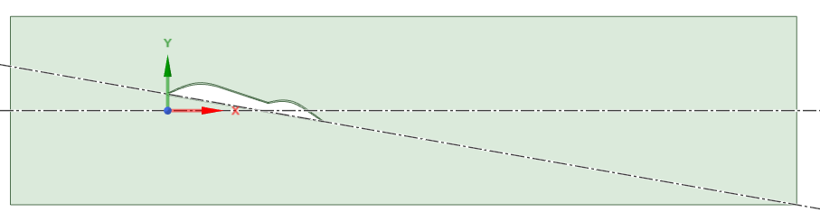
CFD Simulation Setup

• Software: ANSYS Fluent (student Version) was chosen for its robust solver capabilities in aerodynamic analysis.
• Governing Equations: The Navier-Stokes equations, along with turbulence models such as the k−ω SST (Shear Stress Transport), were used to simulate the turbulent flow over the air-foil.
• Meshing: A structured mesh with refinement near the airfoil surface was created to capture boundary layer effects accurately. An inflation layer was used to resolve the near-wall region where high gradients in velocity and pressure exist in ANSYS workbench meshing.

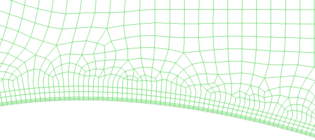
(a) Mesh View near the airfoil surface

 

 

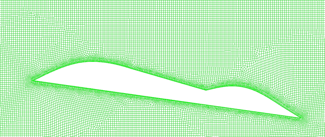
• Boundary Conditions:
  • Inlet: Uniform velocity was applied to represent the free-stream airflow.
  • Outlet: Pressure outlet boundary condition was applied.
  • Symmetry on top and bottom of domain
  • Wall: No-slip boundary condition on the air-foil surface to capture boundary layer development.

Simulation Parameters

• Reynolds Number: The Reynolds number was set at 3×10⁵ to simulate typical air-foil flow conditions for present air foil for air flow at 200 km/hr
• Angles of Attack: The air-foil was analysed at angles of attack of 8° to capture both sub-critical and post-critical conditions for lift and drag.

Results and Discussion

• Computational Fluid Dynamics (CFD) analysis of flow over an airfoil typically involves examining parameters such as pressure distribution, velocity fields, lift, drag forces, and boundary layer development.
• Here’s a breakdown of key aspects of CFD results for this type of analysis:

Pressure Distribution:

• • Upper Surface: The pressure on the upper surface of the airfoil is generally lower than that on the lower surface due to the increased velocity (Bernoulli’s principle), especially near the leading edge. This pressure difference generates lift.
  • Lower Surface: Higher pressure on the lower surface helps contribute to the net lift force.

Velocity Field:

• • Leading Edge: The velocity is highest at the leading edge, where the airflow accelerates to flow over the upper surface.
  • Boundary Layer: The boundary layer develops along the chord length, with changes in its thickness indicating drag characteristics and any possible separation points.

Lift and Drag Coefficients:

• • The Lift Coefficient (Cl) and Drag Coefficient (Cd) are crucial parameters derived from CFD simulations, allowing for the quantification of aerodynamic performance at various angles of attack.
  • These coefficients are often compared against experimental or theoretical values to validate the accuracy of the CFD model.

Flow Separation and Stall:

• • For high angles of attack, CFD results often show flow separation on the upper surface, leading to a stall. This manifests as a reversed or chaotic flow in the velocity field.
  • Identifying the stall angle is critical for assessing the limits of an airfoil’s performance.

Streamlines and Vorticity:

• • Streamline plots illustrate the path of the airflow around the airfoil, highlighting areas of attached flow, separation, and recirculation.
  • Vorticity contours help identify vortex formation and potential instabilities, which are especially relevant for airfoil performance under dynamic conditions.

Pressure Drag and Skin Friction Drag:

• • CFD results allow separate analysis of pressure drag and skin friction drag, providing insights into how the airfoil shape affects overall drag.
  • Skin friction drag is often visible in wall shear stress plots, while pressure drag can be inferred from the pressure distribution and wake structure.

Velocity Contours

(a) Traditional airfoil

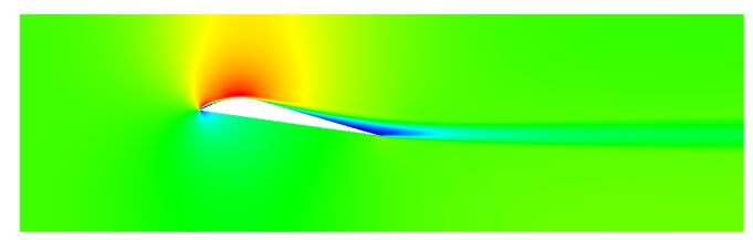
(b) Proposed Double wings air foil

 

 

 

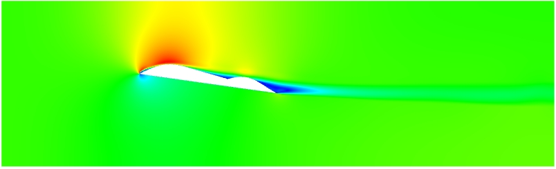
(a) Traditional airfoil

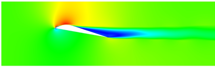
Proposed Double wings air foil

 

 

Pressure Contours

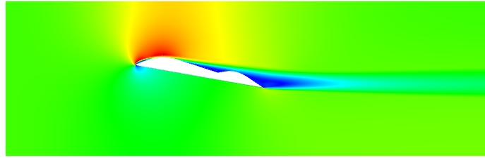
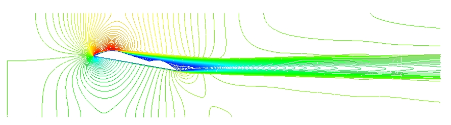
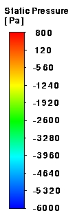
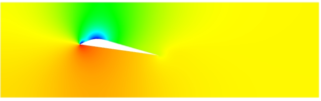
• Pressure contours over an airfoil show how static pressure varies around the airfoil surface and are a direct visualization of lift generation, separation, and stall.
• They are widely used in CFD, wind-tunnel testing, and airfoil design.

(a) Traditional

(b)Double Wing air foil

 

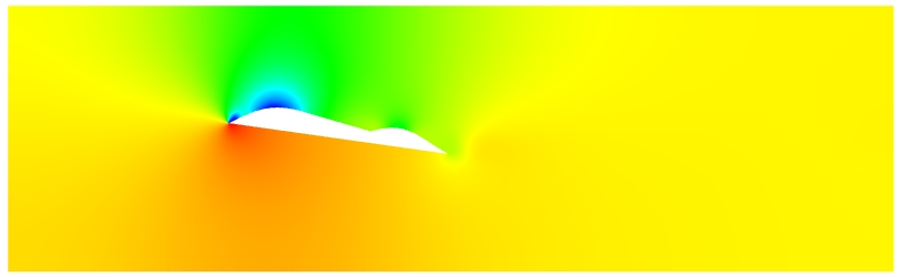
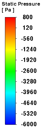
Fig 4. Pressure contours for traditional and proposed air-foils at 200 kmph and AoA = 8°

(a) Traditional

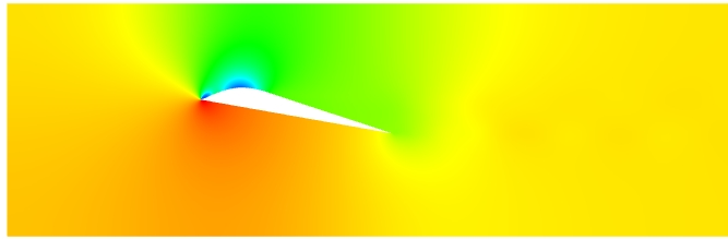
(b) Double wing airfoil

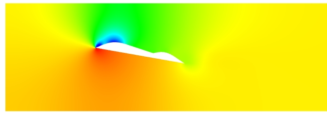
Fig 5. Pressure contours for traditional and proposed air-foils at 200 kmph and AoA = 10°

 

°

Lift Coefficient (Cl)

• The CFD simulations showed that Cl increased almost linearly with angle of attack up to around 12°, after which it reached a peak before starting to decrease, indicating stall. This behaviour was consistent with theoretical and experimental data, validating the CFD model.
• At the critical angle of attack (approximately 12°), separation of the boundary layer from the airfoil’s surface began, causing a loss of lift.
• With an increase in an angle of attack from 8 to 10° the lift coefficient is increased
• With an increase in air speed from 200 to 400 kmph the lift coefficients are increased gradually

Comparison at 200 kmph

Parameter	Traditional Air foil	Proposed air foil	% Difference
Coefficient of Drag, AoA = 8°	0.214	0.208	-3.5%
Coefficient of lift, AoA = 8°	6.9	7.3	6%
Coefficient of Drag, AoA = 10°	0.38	0.34	-9.1%
Coefficient of lift, AoA = 10°	7.3	8.5	16.3%

Comparison at 400 kmph

Parameter	Traditional Air foil	Proposed air foil	% Difference
Coefficient of Drag, AoA = 10°	0.39	0.352	-9.7%
Coefficient of lift, AoA = 10°	7.4	8.6	16.4%

Drag Coefficient (Cd​)

• The drag coefficient Cd was observed to increase gradually with angle of attack. However, around the critical angle, Cd​ increased more sharply due to flow separation and the onset of turbulence.
• The relationship between Cd​ and Cl​ was used to compute the lift-to-drag ratio, indicating the airfoil’s aerodynamic efficiency at each angle of attack.
• With an increase in an angle of attack from 8 to 10° the drag coefficient is decreased

Impact of Flow Conditions

• The CFD model indicated that at higher Reynolds numbers, the airfoil exhibited delayed separation, contributing to a larger Cl and more gradual increase in Cd
• Different turbulence models were tested, and the k−ω SST model provided the closest agreement with experimental data, particularly near stall conditions.

 Conclusion

• The CFD modelling of the drag and lift coefficients for the given airfoil provided accurate and reliable insights into the airfoil’s aerodynamic behaviour. The results were consistent with known experimental data, with the k −ω SST turbulence model effectively capturing the stall and post-stall behaviour. Key findings include:
• The lift coefficient increases with angle of attack until stall, after which lift decreases significantly due to flow separation.
• Drag increases at a faster rate near stall, impacting aerodynamic efficiency.
• CFD proved effective in simulating complex aerodynamic phenomena, providing a cost-efficient alternative to physical testing for preliminary analysis.

References

1. Abbott, I. H., & von Doenhoff, A. E. (1959). Theory of Wing Sections. Dover Publications.
2. Anderson, J. D. (2011). Fundamentals of Aerodynamics. McGraw-Hill Education.
3. ANSYS Fluent Documentation (2024). ANSYS, Inc.